Energy Based Policies

28 Jul 2026

Using energy-based models to represent policies in control and the benefit compared to other commonly used models.

I’ve started to incorporate energy-based models into my own research for learning robot control policies and wanted to share what I’ve learned so far. This blog is intended for other researchers or anyone interested in learning about learning-based policies for robots. I won’t go into depth on model architectures, or exact ways of training. Feel free to check my code for that. I also won’t be implementing flow and diffusion models here, but feel free to check the papers attached and this website for resources. I do hope you gain a high level understanding of the kinds of robot policies out there, and build a solid intuition for how energy-based policies work and why they’re useful.

Recently, there has been some excitement in industry about energy-based models, backed by researchers like Yann LeCun and companies such as Logical Intelligence with their newest KONA reasoning model. Part of what’s appealing is that energy-based models learn a scalar function over candidate solutions, allowing inference to be framed as an optimization problem rather than a purely autoregressive generation process like with large-language models. If we assign low energy to “good” solutions and high energy to “bad” solutions, then finding good solutions boils down to a function minimization problem.

A robot control policy is simply a framework for taking actions given states/observations. We usually denote this policy as \(\pi(a \mid s)\). Here we will focus on a purely offline imitation learning setting where we assume that optimal demonstrations are given in the form of a dataset. The goal is to “imitate” the actions we see in the data while also generalizing well to unseen states.

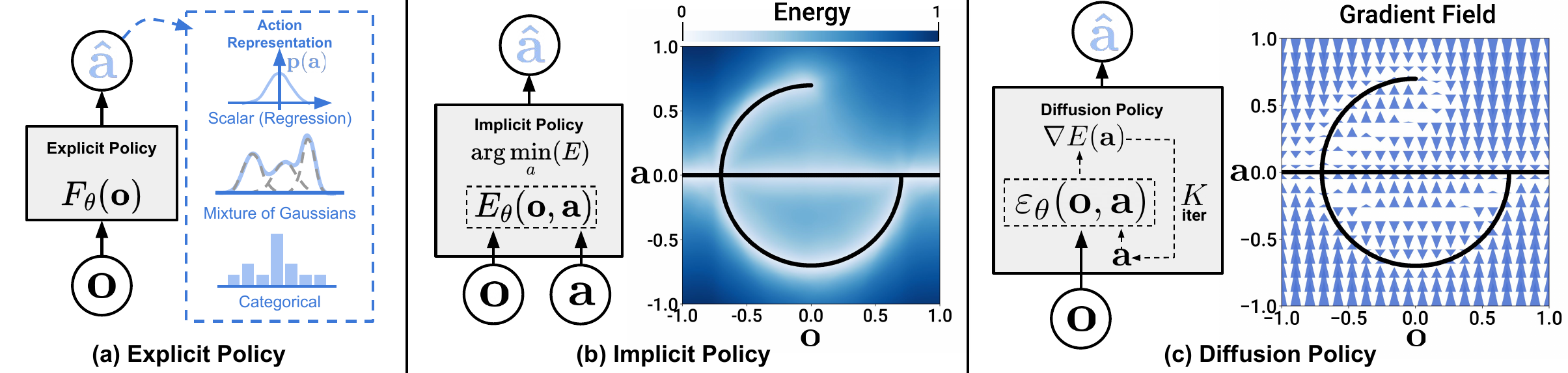
Figure 1: Visualization of different types of policies (source). (a) explicit policies that learn to predict actions directly from observations. (b) Implicit/energy-based policies where optimal actions lie on areas with lowest energy. (c) Iterative generative models refining data from noise.

As of this post, diffusion [6], [3] and score/flow matching [5] models have taken the stage in the robotics community as robot control policies. These models learn noise from data and iteratively denoise to produce outputs that match the data distribution. Our focus today is not these models, but instead energy-based models, or EBMs (middle of Figure 1). Instead of learning a policy directly, EBMs learn an energy function \(E(s, a)\) representing the state-action landscape where our solution space is low energy by construction. Actions can be found at inference time by solving \(a^* = \arg\min_a E(s, a)\). EBMs in continuous, high-dimensional spaces have a reputation for being impractical to train, while diffusion and flow matching policies have a reputation for being easier to learn high dimensional data patterns (e.g. image generation). The go-to objective for EBM-based behavior cloning, implicit behavior cloning (IBC) [1], only reinforces this negative reputation despite extremely impressive results in lower dimensions [3].

First, let me ask you: why bother with EBMs as policies?! We’ve seen diffusion and flow matching do extremely well in the robotics field. My main interest in these energy-based models is composability. Say we train an energy function that pulls a robot arm toward a target. If an obstacle shows up at test time that wasn’t in the training data, we don’t need to retrain anything! We can just add a repulsive energy term that grows large near the obstacle, and minimize the summation of both energies instead. In the real world, this could have profound impacts on safety and interpretability compared to traditional AI controllers being used. I am not here to say that flow and score matching models should not be used. We’ve seen real world robotics problems be solved that we never thought possible with these models! As a researcher, I think it’s always good to take a step back and ask why? Why are these models so good? What knowledge can we take from them? And, maybe most importantly, what is there to gain from trying something different? In my opinion, composability is justification enough to dive deeper.

Methods

Let’s recap the MSE objective and then dive into how IBC and R-NCE work!

Let’s say we are given a dataset \(\mathcal{D}\) of optimal demonstrations of state-action pairs. Vanilla behavior cloning. Vanilla behavior cloning seeks to minimize the mean square error between an offline dataset of optimal actions, and predicted actions from a learned model. We can define a mean-square error objective for the simple vanilla behavior cloning objective. This is extremely simple to implement and with sufficient data can learn reasonable policies. \[\mathcal{L}_{MSE} = \frac{1}{|\mathcal{D}|}\sum_{i \in \mathcal{D}} \|\hat{a}_i - a^*_i\|_2^2 \tag{1}\]

Use your favorite autodifferentiation library and optimizer (e.g. ADAM, SGD) to minimize the MSE. At the end of training, we are given a deterministic policy \(\pi(a \mid s)\) that can predict reasonable actions depending on the task and model capacity. Overfitting to the training data can be common, and often times a regularizer is used to penalize large model weights.

Implicit Behavior Cloning (IBC)

Whereas MSE models would be considered “explicit” policies, energy-based models are “implicit”. Rather than regressing directly to the optimal action, IBC trains \(E_\theta\) with a contrastive, InfoNCE-style loss [1]. For every state-action pair \((s_i, a_i^*)\) in the dataset, we sample \(N_{neg}\) negative “counter-example” actions \(\{\tilde{a}_i^j\}_{j=1}^{N_{neg}}\), and train the model to treat the true action as the lowest-energy option among the batch: \[\mathcal{L}_{InfoNCE} = \sum_{i=1}^N -\log \tilde{p}_\theta\left(a_i^* \mid s_i, \\{\tilde{a}_i^j\\}_{j=1}^{N_{neg}}\right) \tag{2}\] \[\tilde{p}_\theta\left(a_i^* \mid s_i, \\{\tilde{a}_i^j\\}_{j=1}^{N_{neg}}\right) = \frac{e^{-E_\theta(s_i, a_i^*)}}{e^{-E_\theta(s_i, a_i^*)} + \sum_{j=1}^{N_{neg}} e^{-E_\theta(s_i, \tilde{a}_i^j)}}\]

Minimizing this loss encourages the demonstrated action to have lower energy than the sampled counterexamples, i.e. \(E_\theta(s_i, a_i^*) < E_\theta(s_i, \tilde{a}_i^j)\). At inference, once \(E_\theta\) is trained, we can recover the action \(\hat{a} = \arg\min_a E_\theta(s, a)\) using a sampling-based optimizer. Often times a gradient based Langevin dynamics sampler is preferred, but there are also many other ways to sample such as gradient-free cross-entropy methods. \(\eqref{eq:langevin}\) below shows Langevin sampling, which draws samples \(p(a \mid s) \propto e^{-E_\theta(s,a)}\): \[a_{k+1} = a_k - \frac{\lambda}{2} \nabla_a E_\theta(s, a_k) + \sqrt{\lambda}\, \xi_k, \quad \xi_k \sim \mathcal{N}(0, I) \tag{3}\label{eq:langevin}\]

Now, you may be wondering, where do we get counterexamples from?? You’re asking a great question, dear reader! Vanilla IBC assumes that negatives come from a uniform distribution. This simple assumption can work surprisingly well for tasks in low dimensions. Of course, sometimes negatives we sample may be too easy or even meaningless when the dimensionality of the action space increases. We can change the proposal distribution to be a Gaussian, or even learnable in order to find the “hard” negatives, however, the IBC objective becomes biased once we do this. This is where ranking-noise contrastive estimation comes to the rescue.

Ranking-Noise Contrastive Estimation (R-NCE)

Recently, I stumbled upon a paper that identified a subtle problem with the IBC objective [2]. Vanilla IBC assumes that negative actions are sampled from a uniform distribution. If we instead use a non-uniform proposal distribution \(q_\phi(a \mid s)\), the IBC objective becomes biased by learning the density ratio \(p(a \mid s)/q_\phi(a \mid s)\) rather than the expert distribution \(p(a \mid s)\). This means that simply replacing uniform noise with a more useful proposal can change what the EBM learns.

R-NCE fixes this by explicitly accounting for the probability of sampling each negative action under the proposal distribution. All we’re really doing is swapping IBC’s logit \(-E_\theta(s,a)\) for the proposal-corrected logit \(-E_\theta(s,a) - \log q_\phi(a \mid s)\), and reusing the exact same loss form as eq. 2 — just renaming \(\tilde{p}_\theta\) to \(r_\theta\) to reflect the new logit: \[\mathcal{L}_{RNCE} = \sum_{i=1}^N -\log r_\theta\left(a_i^* \mid s_i, \{\tilde{a}_i^j\}_{j=1}^{N_{neg}}\right) \tag{4}\] \[r_\theta\left(a_i^* \mid s_i, \{\tilde{a}_i^j\}_{j=1}^{N_{neg}}\right) = \frac{e^{-E_\theta(s_i, a_i^*)}/q_\phi(a_i^*\mid s_i)}{e^{-E_\theta(s_i, a_i^*)}/q_\phi(a_i^*\mid s_i) + \sum_{j=1}^{N_{neg}} e^{-E_\theta(s_i, \tilde{a}_i^j)}/q_\phi(\tilde{a}_i^j\mid s_i)}\]

This correction allows us to use non-uniform proposals without introducing the same population-level bias. More importantly, it means we can learn a proposal distribution that generates harder and more informative counterexamples rather than relying on uniformly sampled actions.

The authors use a learnable proposal \(q_\phi(a \mid s)\), which, for example, can be trained with maximum likelihood on the demonstration data: \[\mathcal{L}_\phi = -\sum_{(s_i,a_i^*)\in\mathcal{D}} \log q_\phi(a_i^*\mid s_i) \tag{5}\]

In summary, R-NCE lets us learn better negative samples without changing the distribution that the EBM is trying to model [2]. This is huge! And we will see the differences this can make in higher dimensions with the Push-T task.

Result Time!

We’ll go through three simple examples. The first is a synthetic multimodal dataset of 1D states and actions. This is great for visualizing what each method does. The next is coordinate regression, which showcases how EBMs can generalize better with less data compared to a standard MSE loss. Finally, Push-T is our hardest task, where a robot must learn to push blocks into a target given position commands.

Moons Toy Dataset

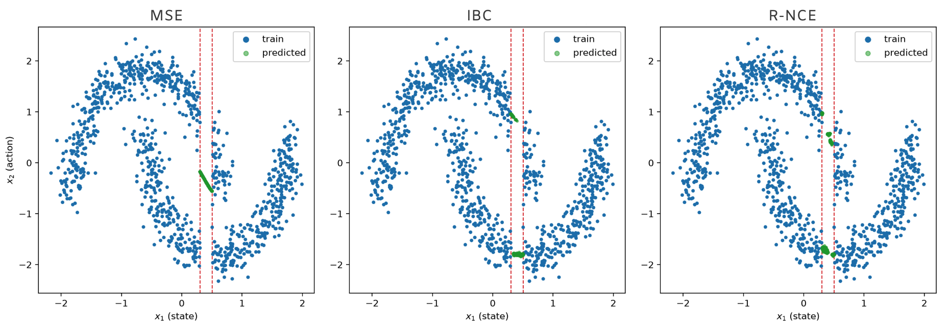
In this example, the X-axis represents states and the Y-axis represents actions. You can see that MSE fails miserably on this task because it can’t handle multimodal data and averages both modes.

Figure 2: Test set action predictions for the moons toy example task. MSE averages both action modes and gives incorrect predictions while energy-based models correctly find multimodal structure in the data.

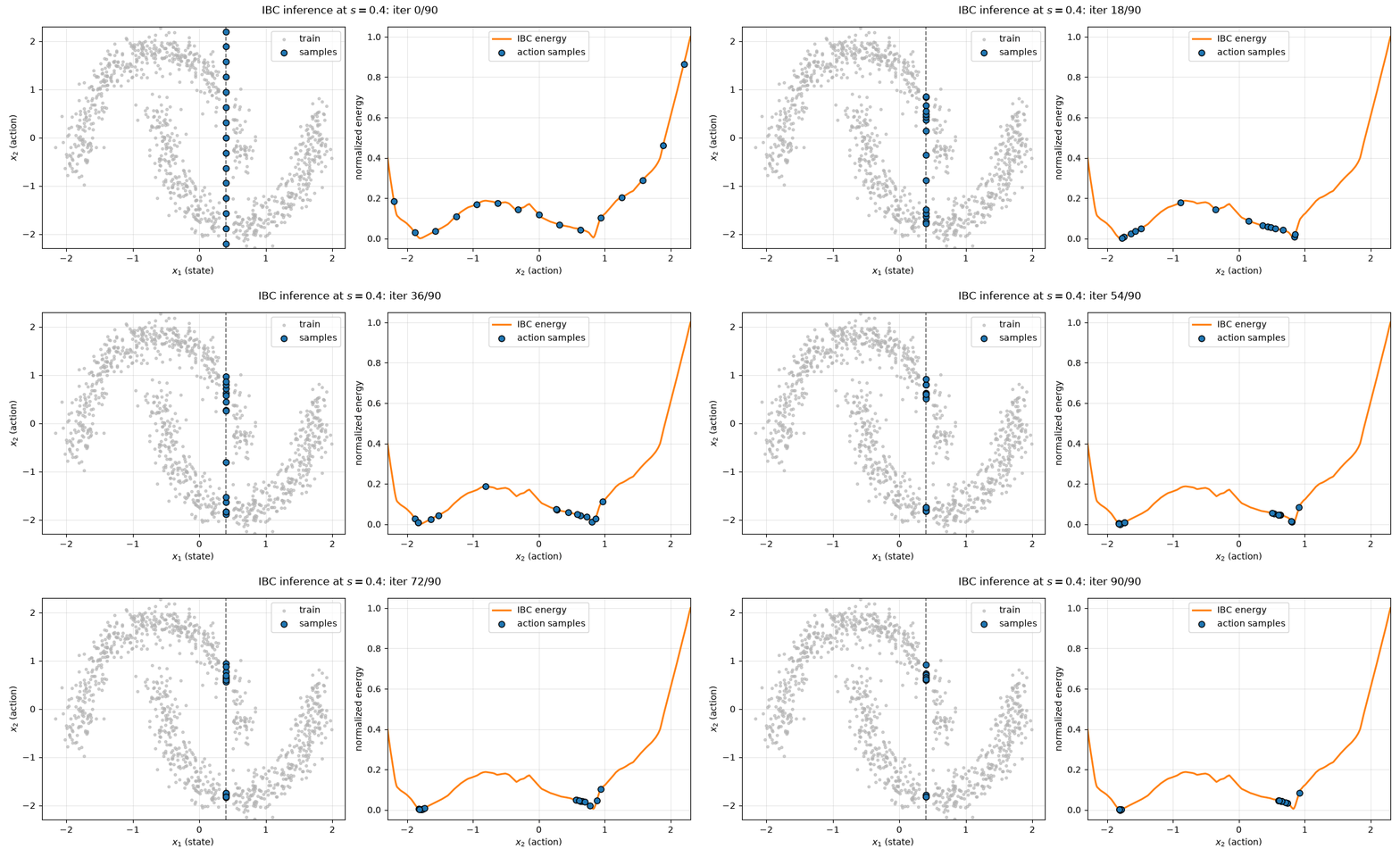
Both EBMs can represent the data and I’ll show you why. Take a look at Figures 3 and 4. These gifs show the final learned energy landscape. Notice the 2 minimums and how the data points iteratively update towards those minimums! Figure 3 uses a uniform proposal distribution and Figure 4 uses the R-NCE objective with a Gaussian proposal policy. In this simple example, both EBMs learn similar energy landscapes, and in fact, a learnable proposal is probably not needed. Notice the dotted purple line in Figure 4? That is the learned proposal mean, and you can see that it is averaging both modes similar to the MSE model we trained. For more complicated tasks, we may want to move away from a simple unimodal Gaussian policy.

Figure 3: Standard energy-based model inference on the moons toy dataset for a held out state of s=0.4. Samples start uniformly over the action space and are iteratively updated with Langevin dynamics.

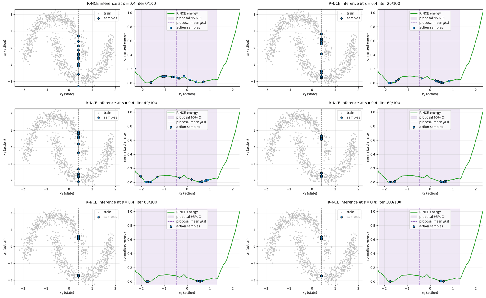
Figure 4: Ranking noise contrastive estimation EBM inference on the moons toy dataset for a held out state of s=0.4. A Gaussian proposal distribution warm-starts the samples and actions are iteratively updated with Langevin dynamics.

Coordinate Regression

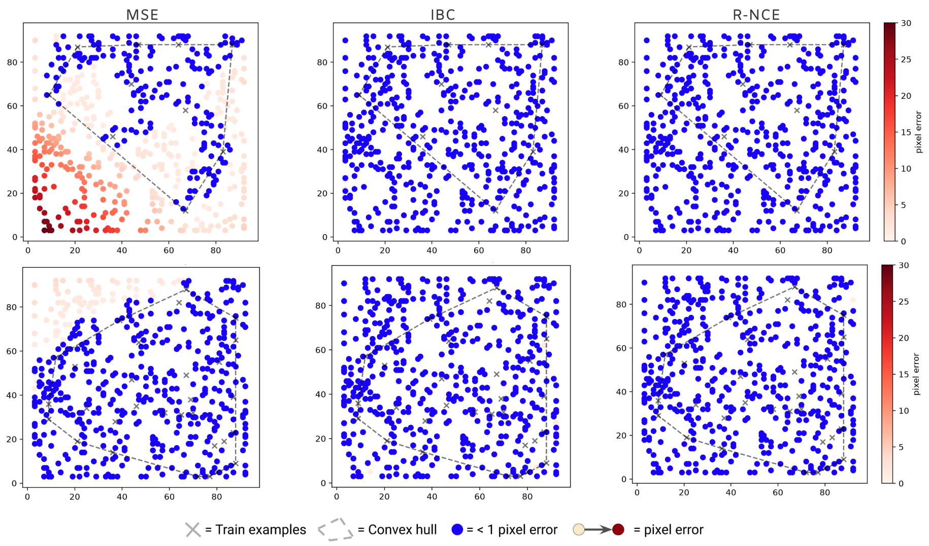
Coordinate regression is a toy vision task introduced in the IBC paper [1]: given an image containing a small, few-pixel green dot, the goal is to regress its \((u, v)\) pixel coordinates. Unlike the rest of this post, this task isn’t about multimodality because there’s only one correct coordinate per image. It’s more about showing spatial generalization with very little data. The IBC authors found that with only 10 training images, an MSE-trained model struggles to even interpolate within the convex hull of the training points, let alone extrapolate outside it. An EBM trained on the exact same handful of images generalizes far better, reporting 1-2 orders of magnitude lower test-set error in this low-data regime. Below I reproduce their setup with \(N=10\) and \(N=30\) training images and show that the gap holds true.

	MSE	IBC	R-NCE
N=10	\(0.368\)	\(0.994\)	\(\mathbf{1.0}\)
N=30	\(0.858\)	\(0.986\)	\(\mathbf{0.994}\)

Figure 5: Test set results for the coordinate regression task. Top: Explicit and implicit models trained on 10 images. Bottom: models trained on 30 images. MSE overfits easily with little training data.

Why do these EBMs generalize better with less data? I would encourage you to read the attached paper more, however, at a high level, the key difference is the implicit function class itself. An explicit MSE model directly represents the mapping \(y=f_\theta(s)\). Models with ReLU activations learn a piecewise-linear function whose output is constrained directly by the training examples. With only a few examples, this can lead to poor extrapolation. An EBM instead represents a continuous energy function \(E_\theta(s,a)\) and obtains its prediction through \(\arg\min_a E_\theta(s,a)\). The IBC authors show that a continuous mapping is forced to pass through every value between two training points. Even though \(E_\theta\) itself is continuous, the \(\arg\min\) used to extract a prediction can jump between disconnected low-energy regions, letting it represent sharp discontinuities directly [1]. This carries over to extrapolation because outside the training data, an implicit model’s prediction tends to continue along whichever piecewise-linear segment of \(E_\theta\) was active nearest the edge of the training domain, rather than extrapolating the output mapping directly.

Push-T

The final task in this blog is a true sequential control problem where an end-effector must push a T-shaped block into a target (green) position [3]. The goal state stays fixed and the end-effector and T-block have random starting positions. The dataset itself is directly from [3], and consists of 20 state dimensions: 9 fixed points on the T-block, and the pusher’s (x, y) position. Note that the original Diffusion policy paper also had a Push-T dataset with image observations. I chose to only use the keypoint-states for simplicity with an MLP, so no CNN or transformer backbones are used. The action is the 2D coordinate for where to move the end-effector to. Internally, a PD controller moves from the current position to the next position.

Score is the max target area coverage averaged over 256 different initial conditions with 5 repeated rollouts, i.e. s = min(coverage / 0.95, 1). On the left hand side of the table below you will see symbols \(T_a\) and \(T_p\). These are the number of executed actions and action predictions. The first row shows scores where we don’t action chunk and predict a single action given the current and previous observation. The last row shows action chunking where 8 actions are executed at once, more similar to diffusion policy execution and model-predictive control settings.

	MSE	IBC	R-NCE
\(T_p=1,\ T_a=1\)	\(0.246 \pm 0.039\)	\(0.570 \pm 0.044\)	\(0.643 \pm 0.044\)
\(T_p=2,\ T_a=2\)	\(0.478 \pm 0.056\)	\(0.237 \pm 0.025\)	\(\mathbf{0.772 \pm 0.041}\)
\(T_p=4,\ T_a=4\)	\(0.667 \pm 0.052\)	\(0.169 \pm 0.024\)	\(0.613 \pm 0.049\)
\(T_p=16,\ T_a=8\)	\(0.632 \pm 0.054\)	\(0.149 \pm 0.022\)	\(0.530 \pm 0.042\)

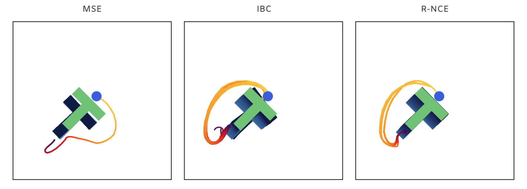
Figure 6: MSE, IBC, and R-NCE rollouts for a fixed initial state. Interestingly, energy-based models don’t use the full multimodal action landscape.

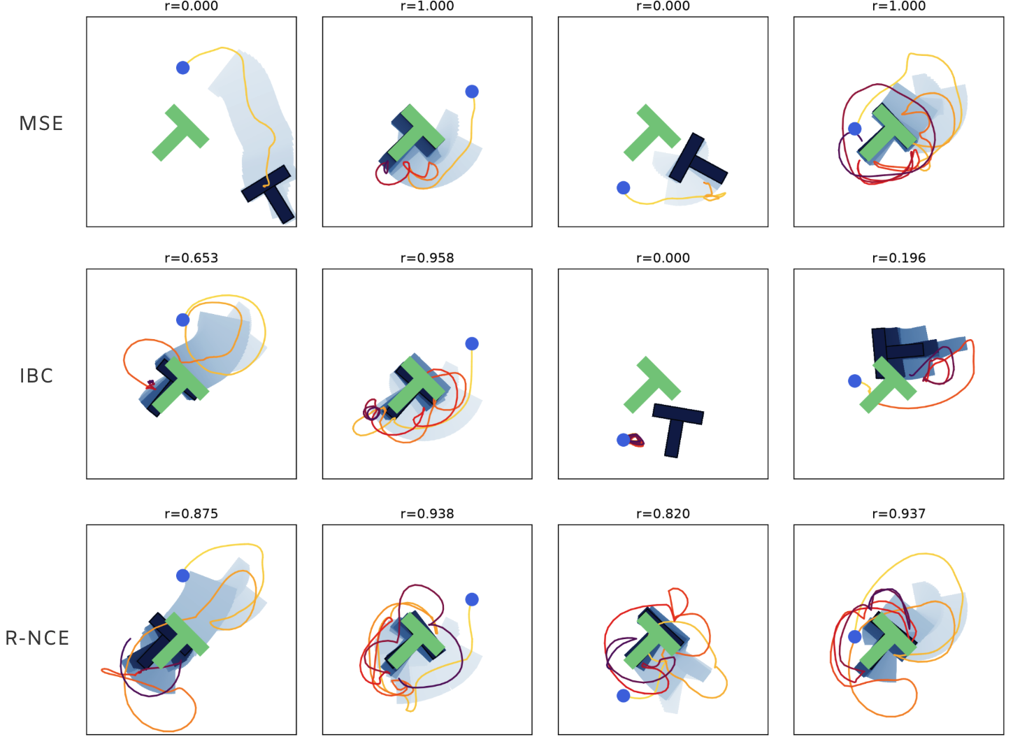
Figure 7: MSE, IBC, and R-NCE rollouts from four test set initial states.

Interestingly, IBC begins to degrade as the action horizon increases, while R-NCE achieves its best performance with an action chunk of 2. MSE improves with longer action horizons and eventually outperforms IBC, suggesting that its smoother predictions are more robust to executing multiple actions open-loop. R-NCE, however, achieves the best overall performance, likely benefiting from its ability to model the multimodal action distribution without the same sensitivity to the negative proposal distribution as IBC. Overall, these results suggest that the choice of negative sampling strategy matters substantially for EBMs in sequential control, particularly as the action horizon grows.

Final Thoughts

I hope you learned a thing or two about EBPs and their difference from explicit policies such as those trained with MSE loss. R-NCE does a much better job in higher dimensions than the standard way of training implicit policies, so let’s not write these models off just yet. Yes, diffusion and flow matching are the new “big thing” in robotics, and yes, they have comparable results with R-NCE [2]. As research in the field progresses, I imagine both energy-based policies and diffusion policies will have their own unique use cases. All we can do for now is stay curious and excited about what is to come!!

If you have any questions or comments, feel free to email me at mat028 [at] ucsd [dot] edu.

Code

Code for this blog is available here: github.com/mht3/ebp.

References

1. Pete Florence, Corey Lynch, Andy Zeng, Oscar Ramirez, Ayzaan Wahid, Laura Downs, Adrian Wong, Johnny Lee, Igor Mordatch, and Jonathan Tompson. “Implicit Behavioral Cloning.” arXiv:2109.00137, 2021. [arXiv]
2. Sumeet Singh, Stephen Tu, and Vikas Sindhwani. “Revisiting Energy Based Models as Policies: Ranking Noise Contrastive Estimation and Interpolating Energy Models.” arXiv:2309.05803, 2023. [arXiv]
3. Cheng Chi, Zhenjia Xu, Siyuan Feng, Eric Cousineau, Yilun Du, Benjamin Burchfiel, Russ Tedrake, and Shuran Song. “Diffusion Policy: Visuomotor Policy Learning via Action Diffusion.” arXiv:2303.04137, 2024. [arXiv]
4. Kevin Zakka. “A PyTorch Implementation of Implicit Behavioral Cloning.” Version 0.0.1, 2021. [GitHub]
5. Yaron Lipman, Ricky T. Q. Chen, Heli Ben-Hamu, Maximilian Nickel, and Matt Le. “Flow Matching for Generative Modeling.” arXiv:2210.02747, 2023. [arXiv]
6. Jonathan Ho, Ajay Jain, and Pieter Abbeel. “Denoising Diffusion Probabilistic Models.” arXiv:2006.11239, 2020. [arXiv]